Tim's Favorite Search Problem
Setup:
The agent has preferences given by \[ \sum_{t}\beta^t c_t \]
-
If the agent is unemployed at the start of the period (state \( S^U \)), then a random wage offer \(w\) is drawn from the fixed distribution \(F(w)\), which has support \([0,B]\). The agent can choose to accept or reject the offer.
- If they accept, they earn income \(w\), and then enter the next period employed at wage \(w\).
- If they reject, they earn fixed income \(b\), and then enter the next period unemployed. Assume \(b \in[0,B)\).
-
If the agent is employed at the start of the period with wage \(w\) (state \(S^E(w)\)), they earn income \(w\), and then enter the next period employed with wage \(w\). Jobs can never be lost.
- Income is in terms of units of consumption, and cannot be saved. There is also no borrowing nor lending, so the agent will consume their income each period.
This system can be summarized by the following diagram. (key)
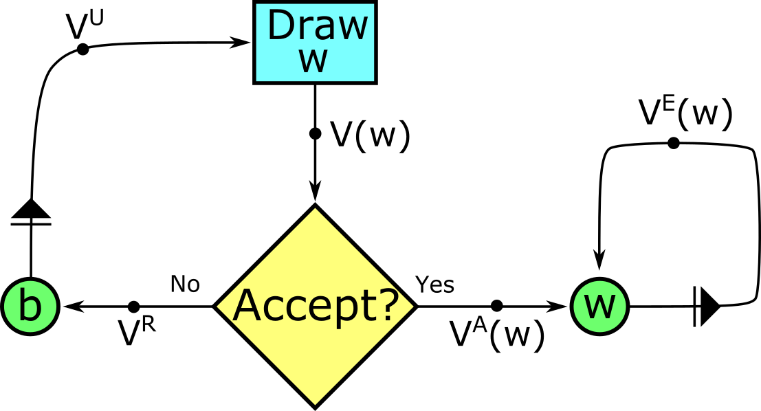 The loop of being employed is on the right, and the loop of searching for a job is on the left. \(V(w)\) is the present value of having offer \(w\) in hand. \(V^U\) is the present value of starting a period unemployed.
Characterizing the Decision Rule
Note that per-period utility flow is bounded, and so with discounting, all present values are bounded as well. At this point, we don't know what these present values are numerically, nor even if they are computable. But by the time-invariance of the process, we know that they exist, and can establish some relationships between them:
\[V^R = b +\beta V^U\]
\[V^U = E[V(w)] \]
\[V(w) = \max \left\{V^A (w),V^R\right\} \]
\[ V^A (w) = V^E (w) = w + \beta V^E (w) = {w \over 1-\beta} \]
It is optimal to accept an offer iff \({w \over 1-\beta}\geq V^R\). The expression \({w \over 1-\beta}\) is strictly increasing in \(w\), and \( V^R\) is constant, though we don't know it yet. By the intermediate value theorem, there must be a reservation wage \(\bar{w}\) such that \({\bar{w} \over 1-\beta}= V^R\) and it is optimal to accept an offer iff \(w\geq\bar{w}\). Therefore:
\begin{split}
V^U = E\left[V(w)\right] & = \Pr(w<\bar{w})V^R & + \Pr(w\geq\bar{w})E\left[{w \over 1-\beta}\mid w\geq\bar{w}\right] \\
V^U = E\left[V(w)\right] & = F(\bar{w})V^R & + \int_{\bar{w}}^{B} {w \over 1-\beta} f(w) dw
\end{split}
\[ {\bar{w} \over 1-\beta} = V^R = b +\beta V^U = b + \beta F(\bar{w}){\bar{w} \over 1-\beta} +\beta \int_{\bar{w}}^{B} {w \over 1-\beta} f(w) dw \]
The above formula characterizes the reservation wage for given \(b\) and \(F\). Rearranging:
\[ 0 = \bar{w}\left({1-\beta F(\bar{w}) \over 1-\beta}\right) -b - \beta \int_{\bar{w}}^{B} {w \over 1-\beta} f(w) dw \]
You can verify that this has only exactly solution by evaluating the right-hand side as a continuous function of \(\bar{w}\). The RHS is negative at \(\bar{w}=0\), positive at \(\bar{w}=B\), and the derivative is strictly positive over \((0,B)\).
Comparative Statics: Increasing Unemployment Benefits \(b\).
Consider two economies with different unemployment benefits \(b_1\) and \(b_2\), but that are otherwise identical.
Let \(b_2 > b_1\). Define:
\[ \hat{b}(x) \equiv x\left({1-\beta F(x) \over 1-\beta}\right) - \beta \int_{x}^{B} {w \over 1-\beta} f(w) dw \]
From above, we know that \(b_i = \hat{b}(\bar{w_i})\). Taking the derivative,
\[ \hat{b}'(x) = \left({1-\beta F(x) \over 1-\beta}\right) - x{\beta\over 1-\beta}f(x) - {\beta\over 1-\beta} (-xf(x)) = \left({1-\beta F(x) \over 1-\beta}\right) > 0\]
So because \(\hat{b}(x)\) is strictly increasing, \(b_2>b_1 \implies \hat{b}(\bar{w_2})>\hat{b}(\bar{w_1}) \implies \bar{w_2} > \bar{w_1} \)
More intuitively, but a bit less rigourously, let \(V^U_i\) be the present value of starting a period unemployed in economy \(i\). We know that \({\bar{w_i} \over 1-\beta} = V^E(\bar{w_i})=b_i+\beta V^U_i\) and so \(\bar{w_i}=(1-\beta)(b_i+\beta V^U_i)\)
Note that \(V_2^U \geq V_1^U\). If the agents in each economy follow the same strategy, and witness the same sequence of random events, then the agent in economy 2 will always have per-period income at least as high as the agent in economy 1. So it can't possibly be that \(V_2^U < V_1^U\). And so:
\[\bar{w_2}=(1-\beta)(b_2+\beta V^U_2) > (1-\beta)(b_1+\beta V^U_1) = \bar{w_1}\]
This makes sense. Higher unemployment benefits make being unemployed a more attractive prospect, increasing the opportunity cost of accepting any given job offer, which means that fewer job offers will be accepted.
Comparative Statics: Riskier Job Market.
Consider two economies with different distributions for job offers \(F_1\) and \(F_2\), but that are otherwise identical.
Let \(F_2\) be a mean-preserving spread of \(F_1\), and let both distributions have support within \([0,B]\). We will prove that the reservation wage is at least as high in economy 2: \(\bar{w_2}\geq\bar{w_1}\)
Definition: Mean Preserving Spread
Let \(F_1\) and \(F_2\) be the distribution functions of random variables \(X_1\) and \(X_2\).
\(X_2\) is a mean preserving spread of (and is 'riskier than') \(X_1\) iff:
-
\(X_1\) and \(X_2\) have the same mean:
\[ E[X_1] = \int_{-\infty}^{\infty}wf_1(w)dw = \int_{-\infty}^{\infty}wf_2(w)dw = E[X_2] \]
-
And \(X_2\) gives more weight to the tails of the distribution:
\[\forall x, \int_{-\infty}^{x} F_2(w) dw \geq \int_{-\infty}^{x} F_1(w) dw\]
Now to apply this definition to the characterizing formula for reservation wage \(\bar{w_i}\), we need to rearrange the integral in a few ways. First, notice that in this environment,
\[ E_i[w] = \int_{0}^{B} {w} f_i(w) dw = \int_{0}^{\bar{w_i}} {w} f_i(w) dw + \int_{\bar{w_i}}^{B} {w} f_i(w) dw \]
\[\therefore \int_{\bar{w_i}}^{B} {w} f_i(w) dw = E_i[w] - \int_{0}^{\bar{w_i}} {w} f_i(w) dw \]
Next, note that \(f(w)dw=dF(w)\), so applying integration by parts:
\[ \int_{0}^{\bar{w_i}} {w} f_i(w) dw = \int_{0}^{\bar{w_i}} {w} dF_i(w) = \left[F_i(w)w\right]_0^{\bar{w_i}} - \int_{0}^{\bar{w_i}} F_i(w) dw = F_i(\bar{w_i})\bar{w_i} - \int_{0}^{\bar{w_i}} F_i(w) dw \]
Putting this together, we have that
\[\int_{\bar{w_i}}^{B} {w} f_i(w) dw = E_i[w] - F_i(\bar{w_i})\bar{w_i} + \int_{0}^{\bar{w_i}} F_i(w) dw\]
And substituting this into the characterizing formula for reservation wage \(\bar{w_i}\):
\begin{split}
{\bar{w_i} \over 1-\beta} & = V_i^R = b +\beta V_i^U = b + \beta F_i(\bar{w_i}){\bar{w_i} \over 1-\beta} +\beta \int_{\bar{w_i}}^{B} {w \over 1-\beta} f_i(w) dw \\
& = b + {\beta \over 1-\beta}F_i(\bar{w_i}){\bar{w_i}} + {\beta \over 1-\beta} \left[ E_i[w] - \bar{w_i}F_i(\bar{w_i}) + \int_{0}^{\bar{w_i}} F_i(w) dw \right]\\
& = b + {\beta \over 1-\beta} \left[ E_i[w] + \int_{0}^{\bar{w_i}} F_i(w) dw \right]
\end{split}
If you are comparing distributions of the form \(F(w,r)\) where \(r\) is a parameter such that riskiness increases as \(r\) increases, then you can take the derivative of both sides with respect to \(r\) and find that \(\bar{w_i}'(r) > 0\). Otherwise:
Recall that the properties of a mean preserving spread imply that \(E_1[w]=E_2[w]\) and that for any value of \(\bar{w}\), \(\int_{0}^{\bar{w}} F_2(w) dw \geq \int_{0}^{\bar{w}} F_1(w) dw\). Then:
\begin{split}
\bar{w_2} - \bar{w_1} & = (1-\beta)b + \beta E_2[w] + \beta \int_{0}^{\bar{w_2}} F_2(w) dw - (1-\beta)b - \beta E_1[w] - \beta \int_{0}^{\bar{w_1}} F_1(w) dw \\
& = \beta \int_{0}^{\bar{w_2}} F_2(w) dw - \beta \int_{0}^{\bar{w_1}} F_1(w) dw \\
& = \beta \int_{\bar{w_1}}^{\bar{w_2}} F_2(w) dw + \beta \int_{0}^{\bar{w_1}} \left[ F_2(w)-F_1(w)\right] dw \geq \beta \int_{\bar{w_1}}^{\bar{w_2}} F_2(w) dw \\
\end{split}
Note that if \(\bar{w_2} \geq \bar{w_1}\), then \(\int_{\bar{w_1}}^{\bar{w_2}} F_2(w) dw \geq 0 \) and \(F_2(\bar{w_1}) \leq F(w)\) for all \(w \in [\bar{w_1}, \bar{w_2}]\).
Likewise, if \(\bar{w_2} \leq \bar{w_1}\), then \(\int_{\bar{w_1}}^{\bar{w_2}} F_2(w) dw \leq 0 \) and \(F_2(\bar{w_1}) \geq F(w)\) for all \(w \in [\bar{w_2}, \bar{w_1}]\). In either case,
\[\bar{w_2} - \bar{w_1} = \beta \int_{\bar{w_1}}^{\bar{w_2}} F_2(w) dw \geq \beta \int_{\bar{w_1}}^{\bar{w_2}} F_2(\bar{w_1}) dw = (\bar{w_2} - \bar{w_1}) \beta F_2(\bar{w_1})\]
\[ \implies (\bar{w_2} - \bar{w_1}) (1 - \beta F_2(\bar{w_1})) \geq 0 \implies \bar{w_2} \geq \bar{w_1} \]
It is also worth noting that a higher optimal reservation wage implies \(V^R_2 > V^R_1\), and so the agent's present value will be at least as high in economy 2 for any given wage offer. Intuitively, when the distribution of wages is spread out, the expected value of accepting a job offer in the next period remains the same; it's just that the chances of very good offers and very bad offers increase. But the agent just ignores the very bad offers.